Part 3: Extracting Kaggle data and building the Convolutional Neural Network (CNN)

Welcome to Part 3 of our tutorial where we will be focused on how to extract our data from the Kaggle set and building our Convolutional Neural Network.

1. Introduction
2. Getting Started
3. Transforming Kaggle Data and Convolutional Neural Networks (CNNs) (Current)
4. Training the neural network
5. Optimising our neural network
6. Converting and Freezing our CNN
7. Quanitising our CNN
8. Compiling our CNN
9. Running our code on the DPU
10. Conclusion Part 1: Improving Convolutional Neural Networks: The weaknesses of the MNIST based datasets and tips for improving poor datasets
11. Conclusion Part 2: Sign Language Recognition: Hand Object detection using R-CNN and YOLO

The Sign Language MNIST Github

Last time we introduced the Sign Language MNIST from Kaggle which consists of 27,455 training images and 7172 test cases, where each test case is a 28×28 greyscale image with pixel values between 0-255. The download we get from Kaggle consists of two csv files: test and train. In each csv the first column is the label with the subsequent columns being the 28×28 pixel values. Our first task is to extract and separate the data from the csv files into training, testing and validation data and labels, which is the standard structure needed to train neural networks in TensorFlow:

• Training data: The data that will be used to train the neural network
• Validation data: Validation data is generally a slice of data taken from the training data. It is not directly used to train the neural network, but is instead used at the end of each epoch to gain results on how well our training is progressing. We can use this data to tune hyperparameters and make decisions on optimising the training process
• Test data: Once a model has been fully trained, we need to test it on data that the model has never been exposed to before, which is the test data. This gives us an indication of what to expect when the model is deployed in the field.

The dataset does not provide a seperate validation set, so we will need to generate some. In general it is recommended to have a ratio of 70% Training data, 15% Validation data and 15% Test data.

Extracting the data

Load the docker platform as before. This time we are going to run the program in a sequence, starting with:

python3 main.py

This file handles the data extraction, training and conversion of the models. main.py performs data extraction by handling the file parsing before using the extract_data.py module to provide the training, validation and testing data and labels:

training_dataset_filepath='%ssign_mnist_train/sign_mnist_train.csv' % dataset_loc
testing_dataset_filepath='%ssign_mnist_test/sign_mnist_test.csv' % dataset_loc
train_data, train_label, val_data, val_label, testing_data, testing_label=extract_data(training_dataset_filepath, testing_dataset_filepath, num_test)

train_data = np.genfromtxt(training_dataset_filepath, delimiter=',')
train_data=np.delete(train_data, 0, 0)
train_label=train_data[:,0]
train_data=np.delete(train_data, 0, 1)

testing_data = np.genfromtxt(testing_dataset_filepath, delimiter=',')
testing_data=np.delete(testing_data, 0, 0)
testing_label=testing_data[:,0]
testing_data=np.delete(testing_data, 0, 1)

train_data = train_data.reshape(27455, 28, 28, 1).astype('float32') / 255
testing_data = testing_data.reshape(7172 , 28, 28, 1).astype('float32') / 255

train_label = train_label.astype('float32')
testing_label = testing_label.astype('float32')

val_data = train_data[-4000:]
val_label = train_label[-4000:]
train_data = train_data[:-4000]
train_label = train_label[:-4000]

train_label = utils.to_categorical(train_label)
testing_label = utils.to_categorical(testing_label)
val_label = utils.to_categorical(val_label)

Building our Convolutional Neural Network (CNN)

Now we have our data ready, let us build our CNN architecture. For MNIST datasets, accurate results can be obtained through the use of Fully Connected layers with no need for convolution layers, but since our dataset is slightly more complex we will be using a full CNN architecture:

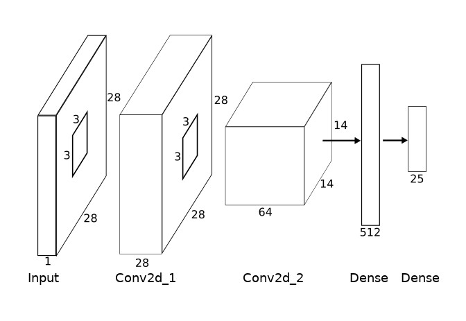
The CNN is described as a Keras model:

def neural_network():
  inputs = layers.Input(shape=(28, 28, 1))
  net = layers.Conv2D(28, kernel_size=(3, 3), padding='same')(inputs)
  net = layers.Activation('relu')(net)
  net = layers.BatchNormalization()(net)
  net = layers.MaxPooling2D(pool_size=(2,2))(net)

  net = layers.Conv2D(64, kernel_size=(3, 3), padding='same')(net)
  net = layers.Activation('relu')(net)
  net = layers.BatchNormalization()(net)
  net = layers.MaxPooling2D(pool_size=(2,2))(net)
  net = layers.Dropout(0.4)(net)
  net = layers.Flatten(input_shape=(28, 28,1))(net)

  net = layers.Dense(512)(net)
  net = layers.Activation('relu')(net)
  net = layers.Dropout(0.4)(net)

  net = layers.Dense(25)(net)

  prediction = layers.Activation('softmax')(net)

  model = models.Model(inputs=inputs, outputs=prediction)
  print(model.summary())
  return(model)

_________________________________________________________________
Layer (type) Output Shape Param # 
=================================================================
input_1 (InputLayer) (None, 28, 28, 1) 0 
_________________________________________________________________
conv2d_1 (Conv2D) (None, 28, 28, 28) 280 
_________________________________________________________________
activation_1 (Activation) (None, 28, 28, 28) 0 
_________________________________________________________________
batch_normalization_1 (Batch (None, 28, 28, 28) 112 
_________________________________________________________________
max_pooling2d_1 (MaxPooling2 (None, 14, 14, 28) 0 
_________________________________________________________________
conv2d_2 (Conv2D) (None, 14, 14, 64) 16192 
_________________________________________________________________
activation_2 (Activation) (None, 14, 14, 64) 0 
_________________________________________________________________
batch_normalization_2 (Batch (None, 14, 14, 64) 256 
_________________________________________________________________
max_pooling2d_2 (MaxPooling2 (None, 7, 7, 64) 0 
_________________________________________________________________
dropout_1 (Dropout) (None, 7, 7, 64) 0 
_________________________________________________________________
flatten_1 (Flatten) (None, 3136) 0 
_________________________________________________________________
dense_1 (Dense) (None, 512) 1606144 
_________________________________________________________________
activation_3 (Activation) (None, 512) 0 
_________________________________________________________________
dropout_2 (Dropout) (None, 512) 0 
_________________________________________________________________
dense_2 (Dense) (None, 25) 12825 
_________________________________________________________________
activation_4 (Activation) (None, 25) 0 
=================================================================
Total params: 1,635,809
Trainable params: 1,635,625
Non-trainable params: 184
_________________________________________________________________