For our introduction to neural networks on FPGAs, we used a variation on the MNIST dataset made for sign language recognition. It keeps the same 28×28 greyscale image style used by the MNIST dataset released in 1999. As we noted in our previous article though, this dataset is very limiting and when trying to apply it to hand gestures ‘in the wild,’ we had poor performance. We can attempt to improve performance by having the images more resemble those used in the ImageNet database, which are higher resolution with colour. We could also improve our accuracy by improving the dataset itself, providing more original data through techniques such as crowd sourcing. With these improvements we may be able to reach the level of technology present in 2012, but we are still left with a AI that has flaws that cannot be fixed with improving the dataset alone, but instead requires us to think of new techniques

• No J or Z: The dataset does not include the letters J or Z as these letters require gesture motions, which is not particularly helpful if we are trying to spell out words. We need an AI that can recognise gesture motions from video. This may also help with the other letters as instead of waiting for the final finished pose, we can get the AI to predict what the next letter will be before the user has made the perfect sign gesture, much like how a human would.
• One hand only please: Our AI was trained with a perfectly cropped image of a single hand, but in actual applications things are rarely this simple. We need to be able to distinguish between multiple hands in the same video and recognise what each hand is doing.

Fortunately, modern techniques allow us to solve both issues to create an AI that could be used outside of a lab environment. Our first intuition is that to recognise J and Z we are going to need temporal information, meaning that we need to know what happened before and after the frame to know if a particular pose corresponds to J or Z. This means that we need an AI that can recognise a hand gesture within a video, which we will call the gesture recognizer. If we feed a neural network a video of multiple hands in it though, this may confuse the AI. Instead we can train a neural network to specifically recognise and localise hands within an image using a bounding box. We can then crop the video according to this localisation and ensure that only one hand is fed into the gesture recognizer. In this part, we will be looking at different CNNs for object detection and localisation.

Recognising and localising hands

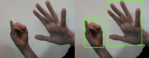
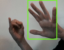
Let us consider this “in the wild” video of a user performing the J gesture motion with one hand, whilst the other hand is in the frame. We need to isolate the two hands and independently check if either of them is performing a sign. We do not just detect if there is an object in the frame, but we also try to find where it is in the image. The easiest way of doing this is training a CNN to not only predict the class of the object but also the position of the object (often in the form of the x y co-ordinates for its centre and also its height and width). This puts extra requirements on our dataset to contain this information, but for now we will assume we have the perfect dataset. This method works nicely if we assume that there is only one hand in our image, but we need to handle multiple hands.

The most intuitive way of detecting multiple hands is through an exhaustive search. We simply sweep windows of different sizes across our image and feed that into a hand detecting neural network. The windows that pass a certain threshold in each region are then classified as objects. The problem though is that multiple windows may detect the exact same hand. To solve this we have our CNN output an additional “objectness” score that estimates the probability of a hand being in the image. We can then find the bounding box with the highest score and remove any overlapping boxes. The problem with this method is that we are sweeping over the entire image multiple times making it very computationally heavy.

Region-based Convolutional Neural Network

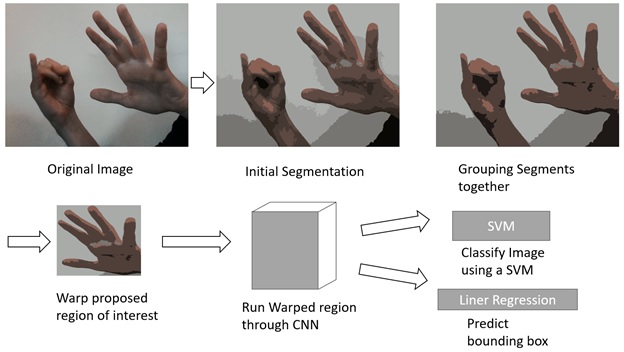
One way of reducing the computations is to be smarter about where we look for objects, which is what Region-based Convolutional Neural Network (2014) or “R-CNN” attempts. Instead of sweeping across the image, we perform a “selective search” on the region. This means that we segment the photo into different regions according to the location and colour. We can then group all these different segments together to form larger regions of interest (ROIs), until we have around ~2K regions. We then reshape these regions into a box that can then be fed into the neural network for prediction. This neural network can be any pre-trained neural network (VGG-16 is a popular choice). We then train an SVM to classify the difference between the object and background. Finally, we decide the bounding box of the object using linear regression. This method required a lot of training of multiple models and also we need to feed around 2000 regions into a neural network making it slow, averaging around 47 seconds per image on a GPU.

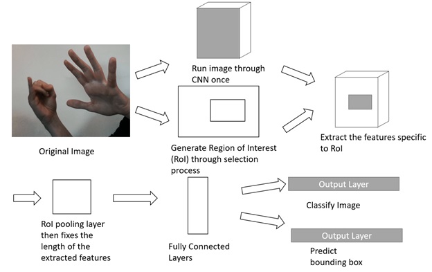
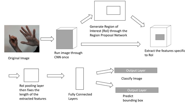
In 2015, “Fast R-CNN” improved this architecture by running the whole image through a feature extraction neural network once rather than running the feature extraction 2000 times. Once we have the outputted feature, we also generate the RoIs as before using the selection process. Using these RoIs we can then extract the features specific to the RoI from the CNN and since the RoI size may vary, the dimensions of the feature map we choose will also vary. We then fix the size by using a RoI pooling layer that fixes the length of the extracted features, before feeding them into the fully connected layers. The fully connected layers then have two outputs: the classifier and bounding box regressor. What is important to notice is that since each learning layer is now connected through fully connected layers, we can do all the learning in one stage as opposed to three. By reducing the amount of times the neural network ran the speeds increased to 2.3 seconds with the majority of the time now being devoted to the selection process.

To increase speeds, the selection process needed to be improved, which was done in 2016 with “Faster R-CNN”, by replacing the selective search with a Region Proposal Network. This network takes as input the feature maps of the CNN and outputs a set of object proposals complete with an objectness score. It works by sliding a small network across the feature maps of the CNN. This network predicts multiple region proposals simultaneously and what the probability of an object being in there is. Each prediction is then made in reference to an anchor box which controls the scale and aspect ratio. The rest of the network remains unchanged. Faster R-CNN forms a single unified trainable network that solves the selective search issue by introducing the region proposal network, increasing speeds to around 0.2 seconds. For embedded purposes though Faster R-CNN is still very large and difficult to run. Whilst Fast R-CNN was being developed, another method called Fully Convolutional Networks was also under work.

Fully Convolutional Network (FCN) and You Only Look Once (YOLO)

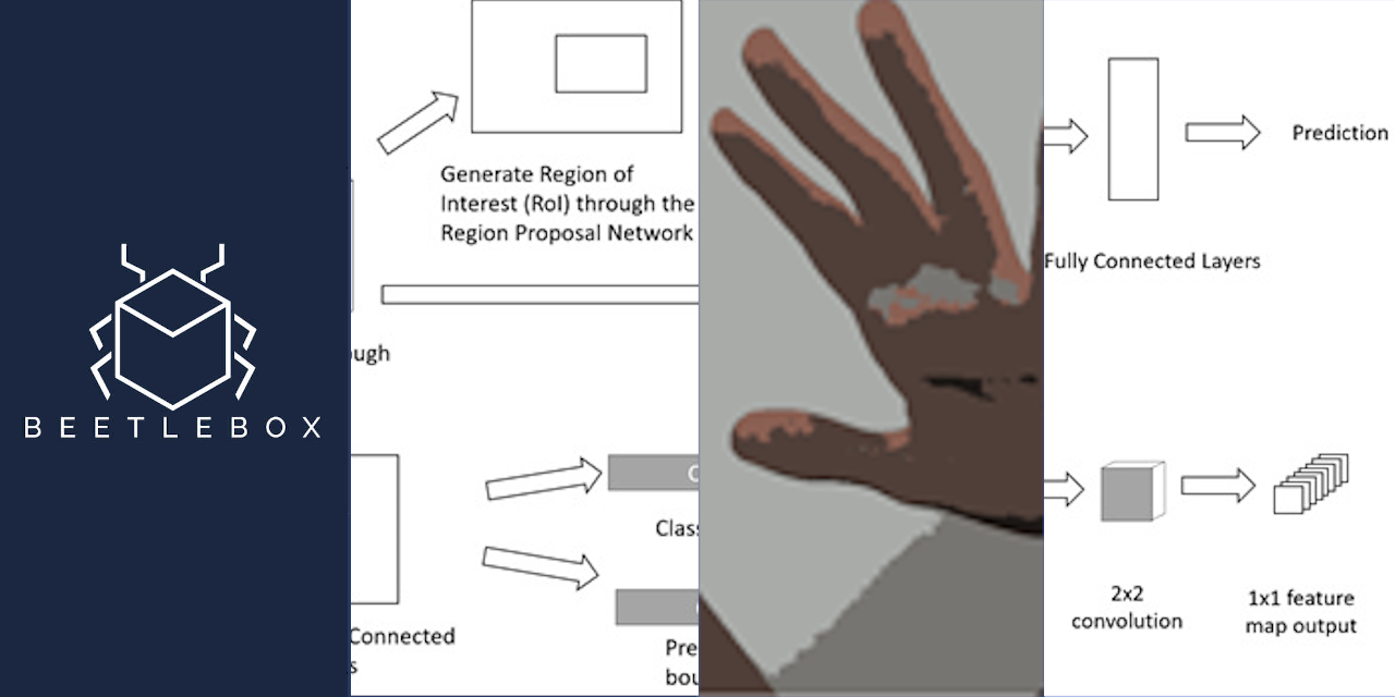
A large problem with R-CNN was that we needed to pass through the image multiple times, but what if it was possible to input an image of any size and run through the image once? The problem we face though is with the fully connected output layers, which need to receive a fixed amount of inputs from the output feature extraction convolutional layer. In 2015, Fully Convolutional Networks were suggested and as the name suggests it replaced all the fully connected layers with convolutional layers instead. This solved the fixed input problem because convolutional layers can use an input of any size. By setting the convolutional layer used for classification to be equal to the size of the final output layer from the feature extraction we can produce a 1×1 feature map output , which has the same output parameters as our previous fully connected layer. This allows our convolutional feature map output to predict: the x,y co-ordinates; width and height; the classification and the objectness score.

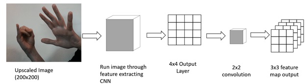
Now we have an output that can handle any size of feature map, we can train our FCN on a small image size (i.e. 100×100) and feed in any other image size. For instance if we have an upscaled image of 200×200, this will double the size of our final feature extraction layer to a 4×4 output layer. This means that our 2×2 convolution for the final output layer will produce a 3×3 feature map output. Essentially, this means that we have reduced the original 200×200 to a 4×4 feature map, which we then use our 2×2 convolution to make predictions on different areas of the image. One of the most popular FCN-based networks is YOLO, which is currently at its third iteration YOLOv3. It has made a few more innovations over a normal FCN, most notably is that the final classification layer does not predict a single bounding box, but predicts five bounding boxes each with its own objectness score. This leads to the bounding boxes specialising in certain sizes, aspect ratios and classifications, improving the overall accuracy. Only needing to perform a single pass leads to significant improvements with the original YOLO able to run at 0.02s which is just the speeds we need to run video in real-time.

Conclusion

To crop out hands from our video, we would recommend the use of YOLOv3 due to its compromise between speed and accuracy. It is based on a single pass through a structure known as a Fully Convolutional Layer, which allows easier training and greater speeds than the other popular method used Faster R-CNN. Faster R-CNN produced an entire system that was achieved through deep learning. It would run the original image and use the outputted feature maps to feed into a Region Proposal Network that would predict RoIs within the image. These RoIs were then reshaped using pooling and fed into fully connected layers where the bounding box and classification were predicted. Previous versions of R-CNN such as Fast CNN did not use a network for proposing RoI, but instead used an analytic method based on grouping pixels of similar colour and location. Although Fast R-CNN did differentiate itself from the original R-CNN by having all its trainable parts within a single system, meaning it could be trained all at once. It also improved performance significantly by only passing the image through the CNN once. The original R-CNN had three different parts that all needed to be separately trained. R-CNN was a significant step forward from exhaustive search approaches that were previously used to find multiple objects within an image. The exhaustive search approach did allow multiple objects to be detected in an image, whereas simpler CNNs were trained to predict the position of a single object within an image by being asked to predict the centre of a bounding box as well as its width and height. Unfortunately, in the wild we are likely to encounter scenarios where multiple hands are present meaning this simple method could not have been used. This exploration has ultimately been to solve our original CNNs problem that it could not handle more than one hand at a time but deploying YOLOv3 as a hand detector will solve this problem. Next time we will look at solving the problem of recognising gesture motions so that we are able to detect J and Z in our alphabet.