Welcome to the 2020.1 version of getting started with computer vision on Vitis on Zynq. The release of 2020.1 saw significant changes from the old 2019.2 version and we thought it would be useful to update this tutorial to reflect the newer version. In this tutorial we will be covering the basics of software development flow on FPGAs and show how much faster Vitis development is compared to more traditional hardware development with a basic “Hello World” example. This tutorial will be a multi-part series covering the basics of getting started with computer vision and Vitis. We will be covering:

• The quick start method
• The scripted build method using Petalinux and XRT
• Understanding the Vitis Development Flow (Current)
• Using OpenCV on the embedded system

We hope these tutorials will be useful for anyone looking to get into computer vision on FPGAs.

Part 3: Understanding the Vitis Development Flow

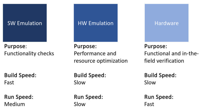
In our previous tutorials, we looked at quickly building the Vector Addition example and then running it on the board. When we want to design something of our own though, we do not want to be constantly building for hardware, which is slow. In traditional Register Transfer Level (RTL) design where we use languages such as Verilog, System Verilog, VHDL, hardware engineers had to constantly build from scratch. It took awhile to build a simple vector addition, enough time to make a coffee. If we had a more complex design, a build could easily take a few hours and we would have enough time to make coffee for the entire office. One of the benefits of developing using Vitis and C-based development flow is that we can check functionality through software emulation, which is an order of magnitude times faster than hardware emulation or running on the system. Once we have the desired functionality, we can then perform hardware emulation to optimise our design in terms of performance and resource usage. Finally, we run the system on the board itself for both functional verification and for in-the-field testing. Running the system on the board allows us to process data far more efficiently, allowing us to check that our system is working for larger amounts of data than emulation can handle.

Software Emulation

Software emulation allows for the quick building of C-based IP that can be tested as software code. When we develop in Vitis, we develop code that runs on the CPU (our host) and code that will be accelerated through the FPGA fabric (our kernels). In software emulation, both the host and kernel code is compiled quickly to be emulated on an x86 system. The advantage of software emulation is not only do we get increases in build speeds, but software emulation speeds are an order of magnitude faster than hardware emulation. The downside is that emulation is far slower than running on the hardware itself, so we probably still want to keep to using low resolution images and videos in software emulation. On top of this we do not get any results on the performance of our kernels, meaning that to optimise our kernels will require us to use hardware emulation. Running our application requires the use of Linux, so Vitis will use the Quick EMUlator (QEMU) to run a Linux system (more information can be found here) and our application will then run on this emulator.

Hardware Emulation

Hardware emulation runs the host code on the QEMU emulator as before, but the kernel code is compiled into RTL code and then runs on the Vivado simulator, providing a cycle accurate view of the kernel code. Since hardware emulation is cycle accurate, there can be differences between it and software emulation, so the first thing we need to ensure is that the hardware emulation gets the same results as the software emulation. The  other major advantage of hardware emulation is that we can gather results on the performance and resource usage of the kernels, allowing us to optimise them for use on the final hardware. We can also use these results to start estimating our actual performance on hardware.

Hardware

Hardware mode provides us with the files we need to run the system on our embedded platform. The host code runs on the ARM processors and the kernels are placed onto the FPGA fabric. This effectively creates the ‘release’ version of our system, enabling us to perform in the field testing. Since hardware runs orders of magnitudes faster than both software and hardware emulation, it can also allow us to perform tests with far larger amounts of data than what is possible in hardware or software emulation. For instance, software emulation may struggle to run a single HD image, but using FPGAs it is possible to process 4K video.

Instructions

Pre-requisites:

• Follow either of the previous two tutorials to have a working system

Our particular setup:

• Operating System: Ubuntu 18.04.04
• Development board tested: ZCU104

Since we are using UBuntu, before we launch Vitis in our terminal we need to set the Libary_Path

export LIBRARY_PATH=/usr/lib/x86_64-linux-gnu
Vitis

Making “Hello World”

To show the differences between the three build modes, we need code that contains both host and kernel code. Vitis provides us with an example program that performs vector addition, so we will use that. Let us begin with a new application program:

Begin from the system project we created last tutorial and create a new application window

• In the Create a New Application Project window:
  • Project Name: hello_world_1
  • Click ‘Next’
• In the Platform window:
  • Click the platform that we created in the previous tutorial
  • Click ‘Next’
• In the Application Project Details window:
  • Set the name to be vec_add
  • Click ‘Next’
• In the Domain window, use the settings options we have used for the previous tutorials
• In the Templates window:
  • Click Vector Addition
  • Click ‘Finish’
• The Vector Addition program consists of three files. vadd.cpp and vadd.h run on the Host, whilst krnl_vadd.cpp runs on the FPGA fabric. Here is an excellent breakdown of how the ‘Vector Addition’ code functions
• To make this a true ‘Hello World’ example, in vadd.cpp let’s add the following line just after the ‘int main(int argc, char* argv[]) {‘ line:

std::cout << "Hello World from Beetlebox"<< std::endl;

Software Emulation

Now that we have modified the code we need to ensure it is functionally correct:

• In the Explorer window, click the vec_add.prj
• In the Application Project Settings, make sure that Active build configuration is set to Emulation-SW as shown below

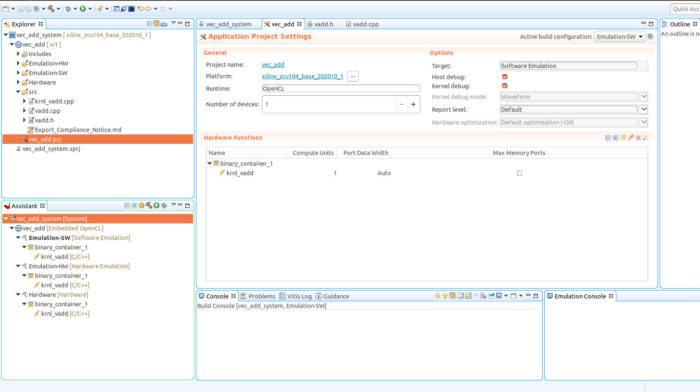
• Build the project
• Once it is built, it is time to debug it. Right Click on vec_add->Run As-> 2 Launch on Emulator (Single Application Debug)
• A window should appear, click Start Emulator and Run
• This will launch the QEMU. A window should appear stating that Vitis is Waiting for the Linux TCF agent to start. In the Emulation Console window, we see Linux booting. Once this has finished (it can take awhile), the program will run
• In the Console window that is titled TCF Debug Process Terminal, we get the following output:

Hello World from Beetlebox
Loading: './binary_container_1.xclbin'
TEST PASSED

• The ‘Emulation Console’ window should be running Linux and we can even rerun our program through the following commands:

cd /mnt/sd-mmcblk0p1
source ./init.sh
./vec_add binary_container_1.xclbin

• Finally, we need to end the emulation: Xilinx->Start/Stop Emulator
• In the Emulation window, hit Stop

Hardware Emulation

Since our code now works in Software Emulation, we should see what the performance and resource usage is through Hardware Emulation as well as testing the functionality.

• In the Explorer window, click the vec_add.prj
• In the Application Project Settings, make sure that Active build configuration is set to Emulation-HW
• Hit build. This process will take far longer than software emulation as the kernels need to be synthesised
• Once built in the Explorer window under vec_add: right click-> run as->run configurations…
• This will open the Run Configurations window. Set Configuration to Emulation-HW. Make sure the emulation box is ticked and then click ‘Run’
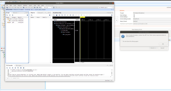
• This will open the Launch on Emulation window, make sure the Launch Emulator in GUI mode to display waveforms is ticked
• The Linux agent will begin to boot before Vivado pops up:

• 
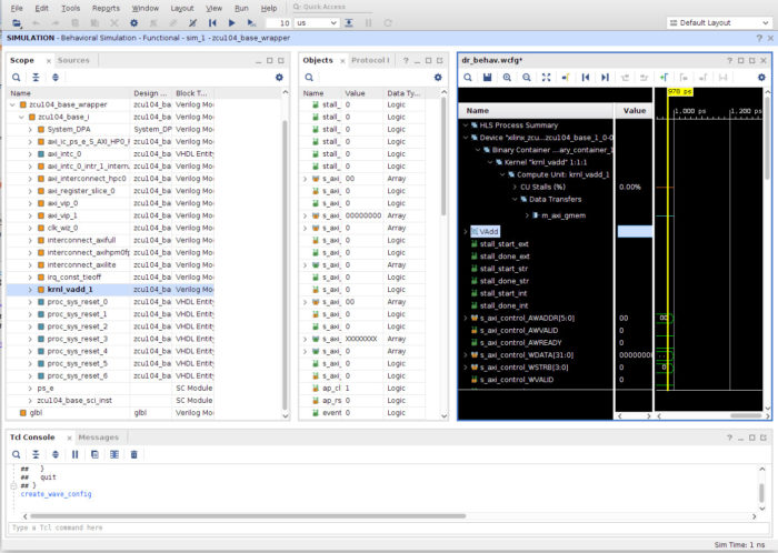
• In the Scope window expand zcu104_base_i
• Right Click on the waveform window and click New Group, call this group VAdd
• Drag krnl_vadd_1 under the VAdd group and then expand to get a view that looks like the following:

• 
• In Vivado, click the Run All button, this will resume the Linux boot sequence in Vitis
• Once Linux is done booting, the program should run and just like in Software Emulation, we should receive the following output from the console

Hello World from Beetlebox
Loading: './binary_container_1.xclbin'
TEST PASSED

• Looking back at Vivado, we should see a distinct area of activity where the kernel was active as shown in the picture below:

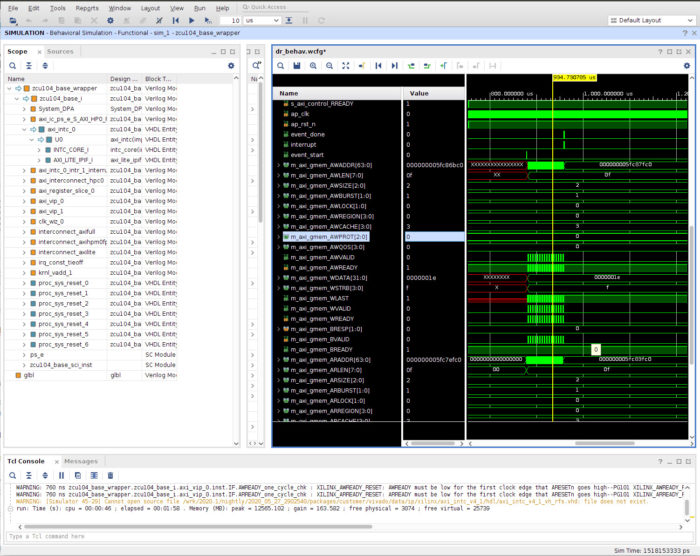
• We can now look at exactly how our kernel is running in hardware in a cycle accurate way, allowing for deeper debugging and a better understanding of how our code is translating into hardware.
• Once we are done, exit Vivado which will automatically stop the emulation as well.
• We can also inspect the performance and resource usage of our modules by using the Vitis Analyzer, which we can launch through a terminal using:

vitis_analyzer

• We can then open the application summary, by hitting Open Summary and finding the following directory:

<workspace_directory>/vec_add/Emulation-HW/binary_container_1.xclbin.link_summary

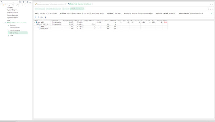
• Using the Vitis Analyzer we can explore in depth the performance and resource usage of our vector addition. At the moment there is not much to explore, but when we are optimizing our own kernels the tools are invaluable.

Hardware

Now we have finished software emulation and hardware emulation, the last thing we need to do is verify that our tool works

• Under the vec_add.prj tab, change Active Build Configuration to Hardware and then hit the build icon.
• When Vitis has finished compiling, it creates a .img file that we are going to flash to our SD card. It is held in the following directory:

<path_to_workspace>/vec_add/Hardware/package/sd_card.img

• This file contains everything the FPGA needs to run our application. Launch balena etcher and select the “sd_card.img” file and then select the SD card, you wish to write to.
• Once your SD card is flashed, check that the Zynq board is in “Boot from SD card mode” and that the board is connected to the host via USB.
• In the Vitis IDE select “Window” > “Show View”, then search terminal and hit “Vitis Serial Terminal.” In the “Vitis Serial Terminal” hit the add button to launch the “Connect to serial port.”
• Keep the default settings the same apart from the port, which will differ depending on the particular host computer.
• Using the Vitis Serial Terminal, we can now run our program as follows:

cd /mnt/sd-mmcblk0p1/
source ./init.sh
./test_2 binary_container_1.xclbin

• We should see the example successfully pass:

Loading: 'binary_container_1.xclbin'
TEST PASSED

In this tutorial we have shown how C-based software development flows can make development of hardware far more efficient. Instead of needing to use RTL where designing, simulating and debugging is very slow, we can use the Vitis Development Environment. Software emulation allows us to quickly verify the functionality of our code, whilst hardware emulation can provide us with the information needed to optimise our kernels as well as check for any functional differences. Finally we can run our code on hardware to verify the functionality of our system and also test using far larger amounts of code. Next time, we will begin exploring using computer vision through running OpenCV on our system.