Part 7: Quantising our graph

In our previous tutorial we produced our frozen model so now we can optimise it to make it run on our FPGA hardware efficiently, which we can do through quantisation. Quantisation is the process of reducing the number of bits used for our tensors and weights, but exactly why is quantisation such a crucial process for FPGAs? The answer lies in their hardware architecture.

1. Introduction
2. Getting Started
3. Transforming Kaggle Data and Convolutional Neural Networks (CNNs)
4. Training our Neural Network
5. Optimising our CNN
6. Converting and Freezing our CNN
7. Quantising our graph (current)
8. Compiling our CNN
9. Running our code on the DPU
10. Conclusion Part 1: Improving Convolutional Neural Networks: The weaknesses of the MNIST based datasets and tips for improving poor datasets
11. Conclusion Part 2: Sign Language Recognition: Hand Object detection using R-CNN and YOLO

The Sign Language MNIST Github

How does quantisation work? The change from floating to fixed

Before we explore quantisation, let’s have a short reminder of the difference between floating and fixed point representation. Chips hold numbers by devoting an amount of binary numbers held in memory. Here is an example of us representing the number four with a four bit memory:

0100

Since we have a set amount of binary numbers, we only have a certain range of whole numbers we can represent (in the case of a signed four bit memory: -(2^3) to (2^3)-1). In CNNs, however, we deal a lot with fractions, which we need to be able to represent. We do this by devoting a certain number of bits to represent the fraction, where each bit after the decimal point represents 2^-n, where n is the position of the bit after the decimal point. For instance to represent 4.125 we could add another four bits to the end of our number:

0100.0010

The precision of the fraction is limited to the number of bits we devote to the fraction. We can remedy this by using floating point, which represents rational numbers. A simplified formula looks like this:

s*2^e

Where a certain number of bits in our memory will represent s or our significand and a certain number will represent e our exponent. Using floating point gives us far greater dynamic range of our numbers, giving us higher precision which in theory should lead to more accurate CNNs. For this reason, most of the time we want to train our CNNs in floating point, but the downside is that the hardware to do floating point arithmetics is more sophisticated.

Quantisation is not just converting between floating to fixed, it is also reducing the number of bits. Floating point tends to be formats that are standardised in a formal process (IEEE 754) and set at either single-precision (32-bit) or double precision (64-bit). Fixed point tends to be more flexible than Floating point because there is only a single way of representing a 7-bit fixed point number. Thus it is a lot easier to experiment with smaller bit-length formats using fixed point. When this is combined with the comparatively simpler arithmetic hardware, it becomes clear why working with fixed point is an appealing option despite the loss of precision.

What about performance degradation?

In most other forms of processing, we can easily find out the performance degradation of using fixed over floating point and use that to inform our choice. What we need to remember with machine learning though is that it is a statistical process meaning that the weights we have trained may not actually be the optimal ones and in fact it is possible that the weights we quantise to produce higher accuracy than the original model, although unlikely. This means that the impact of quantisation on performance is not immediately obvious and there are a lot of studies investigating its impact. Research performed by Qualcomm found that fully connected layers would only start significantly degrading in performance at 6-bits:

http://proceedings.mlr.press/v48/linb16.pdf

In other words, quantising our CNN may not be as detrimental as it sounds. There is also ongoing research into training and retraining quantised models to see if that can help reduce error rates for lower bit lengths

Why do we want to quantise on FPGAs?

In a previous section, we mentioned that one weakness of FPGAs was their limited memory and bandwidth. Quantisation reduces bit lengths and hence reduces memory usage. Going from 32-bit float to 8-bit fixed reduces our memory usage four times, but this is not the end of the story and to show why, we need to take a deeper look into the architecture of our FPGA:

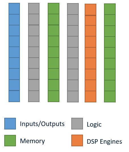
Our FPGA basically consists of columns and columns of a few different types of blocks (IO, Logic, Memory and DSP engines) that are all interconnected. When we program a FPGA, we configure each block and then connect each block up into a specific configuration to represent our hardware (in our case we are configuring it to build our DPU). IO connects our chip to the outside world, whilst our memory blocks contain dedicated RAM for the chip. Logic blocks hold LUTs which implement any logical functions we need. The DSP blocks are our arithmetic powerhouses and to get great performance out of our FPGA requires that we utilise them to their fullest. Let’s take a closer look at a DSP block:

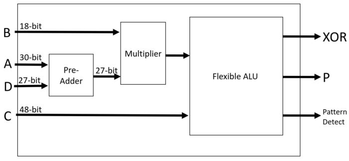
Our DSP block will consist of two DSP slices which can be seen above. The important thing to note here is that the multiplier will only take in a 18-bit and a 27-bit input number, which is less than 32 bits. If we want to do a 32 bit multiplication we need to cascade the result to the next slice below. The ZCU104 has 1,723 DSP slices, if we need to cascade that can effectively halve the number of slices available. This explains why we want to perform convolutions of 18-bit and under, but why do we continue to see benefits at 8-bit? The surrounding logic blocks to the DSP slices are used to feed data in and out. When we lower the bit length, the surrounding logic does not need to be as large, reducing our  bus lengths which helps reduce our LUT usage. In fact, if we lower our bit-length enough, it can become efficient to run the convolutions on the logic blocks themselves, which can increase the amount of processing as there are thousands of LUTs on our device. This is why there is so much interest in running binary and ternary neural networks on FPGAs as it maps very efficiently onto LUTs, massively increasing parallelism.

Quantisation on Vitis AI

With all that theory, it is a relief to know that Vitis AI has made the practical side of quantisation quite simple. Vitis AI converts 32-bit floating point into 8-bit fixed point as this is a good compromise between model accuracy and efficient hardware implementation. Quantisation is not as simple as converting a floating point number to a fixed point number and then chopping off each end evenly to get a 8-bit number. How many bits to give to the fraction is important. Remember that we normalise the inputs to be between 0-1 so to keep as much precision as possible we would prefer to have more bits devoted the fraction, but as we progress along the CNN, that may change. Finding the right balance is important and Vitis AI automates this process for us through calibration. We provide Vitis AI with our training set and it will perform several forward passes devoting different amounts of bits to the fractions and will choose the quantisation scheme that leads to the smallest drop in accuracy. Since we are not performing any back propagation, we do not need too provide any labels either. It is recommended to provide between 100-1000 calibration images.

Implementing quantisation

In our docker run:

vai_q_tensorflow quantize \
--input_frozen_graph=./freeze/frozen_graph.pb \
--input_nodes=input_1_1 \
--input_shapes=?,28,28,1 \
--output_nodes=activation_4_1/Softmax \
--input_fn=image_input_fn.calib_input \
--output_dir=quantize \
--calib_iter=100

testing_data = './sign_mnist_test/sign_mnist_test.csv'
calib_batch_size = 32
testing_data = np.genfromtxt(testing_data, delimiter=',')
testing_data=np.delete(testing_data, 0, 0)
testing_label=testing_data[:,0]
testing_data=np.delete(testing_data, 0, 1)
#testing_data = testing_data.reshape(7172 , 28, 28, 1).astype('float32') / 255
np.savetxt('./quantize/quant_calib.csv', testing_data, delimiter=',')
calib_image_data='./quantize/quant_calib.csv'

def calib_input(iter):
  data = np.loadtxt('./quantize/quant_calib.csv', delimiter=',')
  current_iteration=iter * calib_batch_size
  batch_data=data[current_iteration:current_iteration+calib_batch_size]
  batch_data = batch_data.reshape(calib_batch_size , 28, 28, 1).astype('float32') / 255
  return {"input_1_1": batch_data}

INFO: Calibrating for 100 iterations...
100% (100 of 100) |###################################################################################################| Elapsed Time: 0:04:28 Time: 0:04:28
INFO: Calibration Done.
INFO: Generating Deploy Model...
INFO: Deploy Model Generated.
********************* Quantization Summary *********************      
INFO: Output:       
  quantize_eval_model: quantize/quantize_eval_model.pb       
  deploy_model: quantize/deploy_model.pb

Once we have run the quantisation, we need to see its impact on the accuracy by running our accuracy evaluation again:

Graph accuracy with validation dataset: 0.9295

Now we have performed all the transformations on the graph that are necessary, meaning that next time we can compile the graph to run on our target board and architecture.